Linear algebra with scipy.linalg

In this article, we will see how to use SciPy to perform linear algebra. This article is part of a series on SciPy.

The scipy.linalg module, which implements linear algebra, is a foundational part of the SciPy library. Linear algebra shows up in more places than you might expect. Almost every other SciPy module (such as optimisation, statistics, signal processing, and sparse matrices) uses linear algebra, so a basic understanding of some of the concepts here will help you to get to grips with the other modules too.

You might already know some linear algebra

Linear algebra is the branch of mathematics that covers vectors, matrices, simple curve fitting, and simultaneous equations, amongst other topics. So if you have studied high school maths or beyond, you will already be familiar with some of the concepts.

As a Python programmer, if you've worked with NumPy arrays, you've already been doing linear algebra, even if you didn't call it that. Multiplying two arrays with @, computing a dot product, reshaping data for a model, that's all linear algebra in disguise.

The places where linear algebra crops up in real programming work might surprise you:

• Fitting a line (or curve) to data - least squares is a linear algebra problem
• Solving simultaneous equations - any time you have n unknowns and n equations
• Principal Component Analysis (PCA) - eigendecomposition of a covariance matrix
• Training linear models - gradient descent, normal equations
• Graph analysis - adjacency matrices, PageRank
• Physics and engineering simulations - structural analysis, circuit solving, fluid dynamics

This article is only intended to cover scipy.linalg. It is not a tutorial on linear algebra. But it will include simple summaries of some of the basic concepts, in case your high school maths is a bit rusty.

scipy.linalg vs numpy.linalg - which should you use?

SciPy and NumPy both support linear algebra functions. In many cases, the functions have similar names and give identical results. Which library should you use? It is usually better to choose scipy.linalg, because:

• SciPy has more functions. scipy.linalg offers a richer set of decompositions, matrix functions, and solvers that don't exist in numpy.linalg.
• SciPy gives you more control. SciPy functions often expose more options, such as overwrite_a=True to save memory, or assume_a to hint at matrix structure for performance.
• SciPy has better error handling in edge cases and ill-conditioned matrices.
• LAPACK/BLAS are always available in SciPy. SciPy is always compiled with LAPACK and BLAS support (more on these later). NumPy's linear algebra may or may not be, depending on how it was installed.

The syntax is often identical, which makes switching painless:

import numpy as np
from scipy import linalg

A = np.array([[1.0, 2.0],
              [3.0, 4.0]])

# Both give the same answer - but prefer scipy for serious work
print(np.linalg.det(A))   # -2.0
print(linalg.det(A))      # -2.0

Generally, you should always use scipy.linalg for any serious numerical work. Only use numpy.linalg when you're writing code that deliberately avoids a SciPy dependency (e.g. a lightweight utility library).

The basics - determinants, norms, and the inverse warning

Let's start with the fundamentals before moving on to the more powerful tools.

Determinants

The determinant of a square matrix is a single number that provides basic information about the matrix. In particular:

• If the determinant is zero, then the matrix has no inverse.
• If we use a matrix to transform a shape, then the area of the new shape will be equal to the area of the old shape multiplied by the determinant of the matrix.

For example:

from scipy import linalg
import numpy as np

A = np.array([[3.0, 1.0],
              [1.0, 2.0]])

print(linalg.det(A))  # 5.0  (3*2 - 1*1 = 5, non-singular, good)

B = np.array([[1.0, 2.0],
              [2.0, 4.0]])  # Row 2 is just 2 * Row 1

print(linalg.det(B))  # 0.0  (singular - no unique solution exists)

Norms

The norm of a vector or matrix is a measure of its "size". The default (ord=None) gives the Frobenius norm for matrices (square root of sum of squares of all elements). If the matrix is one-dimensional (ie it is a vector), the Frobenius norm is the length of the vector. For example:

v = np.array([3.0, 4.0])
print(linalg.norm(v))          # 5.0  (classic 3-4-5 triangle)
print(linalg.norm(v, ord=1))   # 7.0  (sum of absolute values)
print(linalg.norm(v, ord=np.inf))  # 4.0  (largest absolute value)

A = np.array([[1.0, 2.0],
              [3.0, 4.0]])
print(linalg.norm(A))          # Frobenius norm ≈ 5.477

The matrix inverse

linalg.inv(A) computes the inverse of a matrix. The inverse of a matrix A is written as:

It has the property that A multiplied by its inverse is the unit matrix I:

Not every matrix has an inverse. For a matrix to have an inverse, it must be square, and it must have a non-zero determinant. Here is an example:

from scipy import linalg
import numpy as np

A = np.array([[3.0, 1.0],
              [1.0, 2.0]])
X = linalg.inv(A)

print(X)   # [[ 0.4 -0.2] [-0.2  0.6]]

Condition numbers

The condition number of a matrix measures how sensitive its determinant is to small changes in the values of the elements of the matrix. A condition number near 1 is ideal. A large condition number (say, 10e+12) means the matrix is nearly singular and your solution may be unreliable.

SciPy doesn't actually provide a cond method. NumPy already has that function in its linalg module, and SciPy doesn't duplicate it. But it is mentioned here because it is useful in this context:

import numpy as np

A_good = np.array([[3.0, 1.0],
                   [1.0, 2.0]])

A_bad = np.array([[1.0, 1.0],
                  [1.0, 1.0001]])  # Nearly singular

print(f"Condition number (good): {np.linalg.cond(A_good):.2f}")   # ≈ 2.62
print(f"Condition number (bad):  {np.linalg.cond(A_bad):.2f}")    # ≈ 40000

As a rule of thumb, if your condition number is of order 10^k, you may lose up to k digits of precision in your solution. For double-precision floating point (about 16 significant digits), a condition number of 10e+12 leaves you with only 4 reliable digits.

Solving linear systems

Solving systems of linear equations is the bread and butter of scipy.linalg. Suppose we have the following set of simultaneous equations:

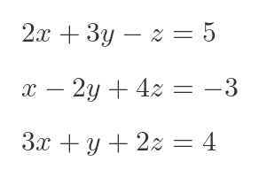
We can represent this as a matrix. Given a matrix A and a vector b, find x such that:

In the case above, A would contain the coefficients of the LHS, and b would contain the values from the RHS:

A = np.array([[ 2.0,  3.0, -1.0],
              [ 1.0, -2.0,  4.0],
              [ 3.0,  1.0,  2.0]])

b = np.array([5.0, -3.0, 4.0])

linalg.solve() - the standard case

For simple cases, where A is square (ie the number of equations is the same as the number of variables), and the determinant of A is not zero, solve() is your go-to function. Under the hood, it uses LU decomposition (more on that shortly), but you don't need to worry about that, just give it A and b.

from scipy import linalg
import numpy as np

x = linalg.solve(A, b)  # Using A and b from before
print(x)  # [ 3,  -1,   -2] approximately

# Always worth verifying your solution
print(np.allclose(A @ x, b))  # True

If you know something about the structure of your matrix, you can give solve() a hint using the assume_a parameter. Supplying a hint can significantly improve performance for large matrices:

# For symmetric matrices
x = linalg.solve(A, b, assume_a='sym')

# For symmetric positive definite matrices
x = linalg.solve(A, b, assume_a='pos')

# For general matrices (default)
x = linalg.solve(A, b, assume_a='gen')

If you aren't sure what type of matrix you have (or what a positive definite matrix even is), then it is best not to supply this parameter, as it could do more harm than good.

You can also solve multiple right-hand sides in one call by passing a matrix instead of a vector for b:

# Solve Ax = b1 and Ax = b2 simultaneously
B = np.array([[1.0, 4.0],
              [-2.0, 1.0],
              [10.0, 5.0]])

X = linalg.solve(A, B)  # X[:,0] solves for b1, X[:,1] solves for b2

linalg.lstsq() - when you have more equations than unknowns

In the real world, data can be messy. You might have more observations than unknowns - for example, 100 data points but only 3 model parameters. That is called an overdetermined system, and there's no exact solution. Instead, lstsq() finds the x that minimises the value of:

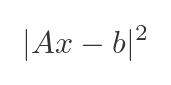
This code finds the classical least-squares solution:

# Fit a straight line y = mx + c to some noisy data
# This is an overdetermined system: many points, two unknowns (m, c)

x_data = np.array([0.0, 1.0, 2.0, 3.0, 4.0, 5.0])
y_data = np.array([1.1, 2.9, 5.2, 6.8, 9.1, 11.0])  # noisy y ≈ 2x + 1

# Build the design matrix [x, 1] for the model y = mx + c
A = np.column_stack([x_data, np.ones(len(x_data))])

solution, residuals, rank, singular_values = linalg.lstsq(A, y_data)
m, c = solution
print(f"Slope: {m:.4f}, Intercept: {c:.4f}")  # Slope: 1.9914, Intercept: 1.0381

scipy.linalg also provides solve_banded() and solve_triangular(), which are useful in the special cases where the matrix is known to be banded or triangular. These are significantly faster than the general solver when applicable, which matters a lot for large systems.

Matrix decompositions

Decomposing a matrix (sometimes called factorising the matrix) breaks a matrix down into simpler, structured pieces. Think of it like factorising a number:

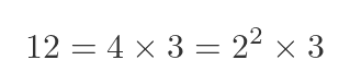
A matrix decomposition produces two or more matrices that, when multiplied, yield the original matrix. Unlike numbers, there are many ways to factorise a matrix.

The benefit of decomposition is that it can speed up certain calculations. For very large matrices, this can make a huge difference in the time taken to perform the calculation. Doing the same calculation without decomposing the matrix will give the same result, but it might take much longer.

Different decomposition methods are useful for different purposes, but using the wrong decomposition can make things worse. If you need to process large matrices, it is worth researching and experimenting to find a suitable decomposition.

LU decomposition - linalg.lu()

LU decomposition splits a matrix A into three factors:

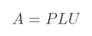
where P is a permutation matrix (just reorders rows), L is lower triangular, and U is upper triangular. Triangular systems are very fast to solve - that's why this is useful.

A = np.array([[2.0, 1.0, 1.0],
              [4.0, 3.0, 3.0],
              [8.0, 7.0, 9.0]])

P, L, U = linalg.lu(A)

print("P:\n", np.round(P, 4))
print("L:\n", np.round(L, 4))
print("U:\n", np.round(U, 4))

# Verify: P @ L @ U should reconstruct A
print(np.allclose(P @ L @ U, A))  # True

QR decomposition - linalg.qr()

QR decomposition splits A into:

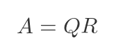
where Q is an orthogonal matrix (Q^T Q = I) and R is upper triangular. It's a good choice for least squares problems and is numerically very stable.

A = np.array([[1.0, 2.0],
              [3.0, 4.0],
              [5.0, 6.0]])

Q, R = linalg.qr(A, mode='economic')  # 'economic' gives compact form

print("Q shape:", Q.shape)  # (3, 2)
print("R shape:", R.shape)  # (2, 2)
print("Orthogonal check:", np.allclose(Q.T @ Q, np.eye(2)))  # True

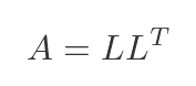
Cholesky decomposition - linalg.cholesky()

The Cholesky decomposition only works for symmetric positive definite matrices (that is, matrices where all the eigenvalues are positive). It is roughly twice as fast as LU decomposition. Covariance matrices in statistics and stiffness matrices in engineering are both symmetric positive definite, so this comes up more than you might expect.

The decomposition uses a lower triangular matrix L, chosen such that L multiplied by its transpose is equal to the original matrix A:

# A covariance matrix is always symmetric positive definite
cov = np.array([[4.0, 2.0],
                [2.0, 3.0]])

L = linalg.cholesky(cov, lower=True)
print("L:\n", L)

# Verify: L @ L.T should recover the original matrix
print(np.allclose(L @ L.T, cov))  # True

# Efficient solve using Cholesky
b = np.array([1.0, 2.0])
c, low = linalg.cho_factor(cov)
x = linalg.cho_solve((c, low), b)
print(x)  # Same as linalg.solve(cov, b) but faster

Singular value decomposition (SVD) - linalg.svd()

SVD is the most powerful and general of all the decompositions. It works on any matrix - not just square ones - and decomposes it as:

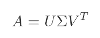
where U and V are orthogonal matrices and Σ is a diagonal matrix of singular values (always non-negative, sorted in descending order).

The singular values tell you how much "energy" or "information" is carried by each component of the matrix. These values form the foundation of PCA, low-rank approximations, and pseudoinverses.

A = np.array([[1.0, 2.0, 3.0],
              [4.0, 5.0, 6.0],
              [7.0, 8.0, 9.0],
              [10.0, 11.0, 12.0]])

# full_matrices=False gives the compact ('economy') form - usually what you want
U, s, Vt = linalg.svd(A, full_matrices=False)

print("Singular values:", np.round(s, 4))  # e.g. [25.4624  1.2907  0.    ]
print("U shape:", U.shape)   # (4, 3)
print("Vt shape:", Vt.shape) # (3, 3)

# Reconstruct A from its factors
A_reconstructed = U @ np.diag(s) @ Vt
print(np.allclose(A, A_reconstructed))  # True

A classic application of SVD is low-rank approximation. You can approximate a matrix using only its top k singular values, discarding the rest. The result is the best possible rank-k approximation to the original matrix:

# Keep only the top k singular values - a rank-k approximation
def low_rank_approx(A, k):
    U, s, Vt = linalg.svd(A, full_matrices=False)
    # Zero out all but the top k singular values
    s_reduced = s.copy()
    s_reduced[k:] = 0
    return U @ np.diag(s_reduced) @ Vt

# For our 4x3 matrix, a rank-1 approximation captures most of the structure
A_approx = low_rank_approx(A, k=1)
print(np.round(A_approx, 2))

# How much of the "energy" does rank-1 capture?
U, s, Vt = linalg.svd(A, full_matrices=False)
print(f"Rank-1 captures {s[0]**2 / np.sum(s**2) * 100:.1f}% of variance")
# ≈ 99.9% - this particular matrix is nearly rank-1

Eigenvalues and eigenvectors

An eigenvector of a matrix A is a special vector v that, when multiplied by A, only gets scaled - it doesn't change direction:

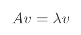
The scaling factor λ is the corresponding eigenvalue. These appear in an enormous range of applications: vibration modes in mechanical structures, stability analysis of dynamical systems, Google's PageRank algorithm, and PCA.

linalg.eig() - general matrices

A = np.array([[4.0, -2.0],
              [1.0,  1.0]])

eigenvalues, eigenvectors = linalg.eig(A)
print("Eigenvalues:", eigenvalues)   # [3.+0.j  2.+0.j]
print("Eigenvectors:\n", eigenvectors)
# Each column is an eigenvector

# Verify Av = λv for the first eigenpair
v0 = eigenvectors[:, 0]
lambda0 = eigenvalues[0]
print(np.allclose(A @ v0, lambda0 * v0))  # True

Note that eig() always returns complex arrays, even when the eigenvalues are real (as above). If you know your eigenvalues should be real, you can safely take the real part:

real_eigenvalues = eigenvalues.real

linalg.eigh() - symmetric matrices (prefer this when applicable)

If your matrix is symmetric (or Hermitian for complex matrices), use eigh() instead. It's faster, more numerically stable, and it always returns real eigenvalues without needing to extract the real part manually.

# A symmetric matrix (e.g. a covariance matrix)
C = np.array([[4.0, 2.0, 0.0],
              [2.0, 3.0, 1.0],
              [0.0, 1.0, 2.0]])

eigenvalues, eigenvectors = linalg.eigh(C)
print("Eigenvalues:", eigenvalues)   # Real values, sorted ascending
# e.g. [0.8787  3.0000  5.1213]

# Eigenvectors are orthonormal - a nice property of symmetric matrices
print(np.allclose(eigenvectors.T @ eigenvectors, np.eye(3)))  # True

The eigenvectors of a covariance matrix are exactly the principal components used in PCA - the directions of maximum variance in your data.

linalg.eigvals() - when you only need the values

If you don't need the eigenvectors, eigvals() is faster:

# Just the eigenvalues - no eigenvectors computed
vals = linalg.eigvals(A)

Matrix functions

You can apply mathematical functions to matrices. Not element-by-element, but in a genuine matrix sense. We typically do this using the Taylor series, but applying it to a matrix rather than a single value. For example, we can apply the exponential function to a matrix A like this:

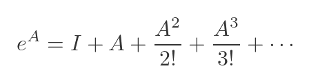
We are using the standard Taylor expansion of the exponential function. We can do this because a square matrix can be raised to an integer power by repeated multiplication. The result is a matrix that has the same dimensions as A.

This is completely different from applying np.exp() to each element.

linalg.expm() - the matrix exponential

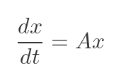
The matrix exponential is used to solve systems of linear ODEs, in control theory, and in quantum mechanics. If you have the system:

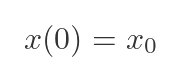
With an initial condition:

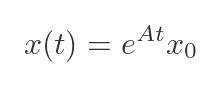
The solution is:

Here is the code:

# System of ODEs: dx/dt = Ax
# x(t) = expm(A*t) @ x0

A = np.array([[-1.0,  0.5],
              [ 0.5, -2.0]])

x0 = np.array([1.0, 0.0])  # initial condition

# Evaluate the solution at t = 0, 0.5, 1.0, 2.0
for t in [0.0, 0.5, 1.0, 2.0]:
    x_t = linalg.expm(A * t) @ x0
    print(f"t={t:.1f}: x = {np.round(x_t, 4)}")

# t=0.0: x = [1. 0.]
# t=0.5: x = [0.6228 0.1206]
# t=1.0: x = [0.4024 0.1211]
# t=2.0: x = [0.1766 0.0681]

Other matrix functions

import numpy as np
from scipy import linalg

# A positive definite matrix for demonstration
A = np.array([[4.0, 2.0],
              [2.0, 3.0]])

# Matrix square root: sqrtm(A) @ sqrtm(A) ≈ A
sqrt_A = linalg.sqrtm(A)
print(np.allclose(sqrt_A @ sqrt_A, A))  # True

# Matrix logarithm: the inverse of expm
log_A = linalg.logm(A)
print(np.allclose(linalg.expm(log_A), A))  # True

# Apply an arbitrary function to a matrix via its eigendecomposition
# e.g. compute sin(A) in the matrix sense
sin_A = linalg.funm(A, np.sin)

These aren't fast for large matrices - they're O(N^3) at best - but for small matrices in physics simulations, control theory, or quantum computing, they're invaluable.

Under the hood: BLAS and LAPACK

You'll hear these names from time to time, so it's worth knowing what they are. BLAS (Basic Linear Algebra Subprograms) and LAPACK (Linear Algebra PACKage) are libraries of highly optimised numerical routines, originally written in Fortran, that have been refined over decades. When you call linalg.solve(), what you're really doing is calling a well-tested LAPACK routine via a clean Python interface.

SciPy exposes direct access to these routines via scipy.linalg.blas and scipy.linalg.lapack, but you will almost certainly never need to go there. The high-level interface handles everything for you.

What you should care about is making sure your NumPy and SciPy are linked to an optimised BLAS implementation. You can check this with:

import numpy as np
np.show_config()

Look for OpenBLAS or Intel MKL in the output. If you installed SciPy via conda, you almost certainly already have a well-optimised setup.

Practical tips and pitfalls

Here are the key lessons to take away:

Never invert a matrix to solve a system. Use linalg.solve(A, b) instead of linalg.inv(A) @ b. It's faster and numerically more stable. The only time you legitimately need inv() is when you actually need the inverse matrix itself.

Check your condition number for ill-conditioned systems. Before trusting a solution, especially with real-world data, call linalg.cond(A). A condition number above 10^{10} or so might be a red flag. Consider regularisation techniques (like Tikhonov regularisation) if your system is ill-conditioned.

Use eigh() not eig() for symmetric matrices. eigh() is faster, always returns real eigenvalues, and guarantees orthonormal eigenvectors. If you know your matrix is symmetric, there is no reason to use eig().

Use lu_factor() + lu_solve() for repeated solves. If you're solving the same system with many different right-hand sides, factorise once and solve many times. This is a very common pattern in numerical simulation.

Use full_matrices=False in SVD. For a matrix of shape (m \times n) with m > n, the full U matrix is (m \times m) - mostly wasted space. The compact form (full_matrices=False) gives you a (m \times n) U matrix and is almost always what you want.

Watch out for overwrite_a=True. Many scipy.linalg functions accept an overwrite_a=True parameter, which allows them to modify the input array in place to avoid a memory copy. This is a useful performance optimisation for large matrices, but it will destroy your input array. Only use it when you no longer need the original.

Further reading

• SciPy linalg documentation
• Linear Algebra and Its Applications - Gilbert Strang (the classic textbook)
• Numerical Linear Algebra - Trefethen & Bau (more advanced, highly recommended)
• MIT 18.06 Linear Algebra - Gilbert Strang's legendary free lecture series
• Scipy Lecture Notes - Linear Algebra