Numerical integration in Python with scipy.integrate - quad, dblquad and sampled data

Numerical integration exists to solve a fundamental problem. Many integrals encountered in real-world physics, engineering, statistics, and finance do not have closed-form antiderivatives. Even when they do, evaluating them symbolically can be computationally expensive or intractable for complex functions. scipy.integrate provides battle-tested, high-performance implementations of classical numerical methods (many wrapping decades-old Fortran libraries like QUADPACK and ODEPACK) so you don't have to implement these methods from scratch.

The module splits neatly into two conceptual halves:

• Approximating definite integrals, either from a known function or from discrete sampled data.
• Solving ordinary differential equations (ODEs), either an initial value problem or a boundary-constrained problem.

This distinction matters because the underlying algorithms are completely different. Approximating a definite integral involves evaluating a function at carefully chosen points and combining the results with weights. At the same time, ODE solvers take discrete steps through "time" (or whatever the independent variable represents), using local error estimates to adapt step size.

What is covered in this article

We will look at:

• quad - the main method used for integrating mathematical functions.
• dblquad. tplquad and nquad - used double, triple, and n-dimensional integration.
• How to handle improper integrals, singularities, and discontinuities.
• fixed_quad for faster, non-adaptive integration.
• trapeziod for integrating sampled functions.
• simpson for integrating sampled functions using quadratic fitting.
• cumulative_trapezoid and cumulative_simpson for finding the cumulative integral of sampled functions.

This article assumes you are comfortable with Python functions, the basics of NumPy arrays, and the calculus concepts of derivatives, definite integrals, and initial-value problems. No prior SciPy experience is assumed.

Setting up

Assuming NumPy and SciPy are both installed, we need the following imports to start using scipy.integrate:

import numpy as np
from scipy import integrate

Many functions in the integrate module accept a Python callable as the primary argument. This will typically be a function f(x) or f(t, y) that you define yourself, often using NumPy operations so it can be vectorised. Inputs and outputs are generally NumPy-compatible.

A key design pattern used throughout the integrate module is that many functions return a bundle of results rather than a single number. For instance, the quad function, which we will look at next, returns (value, error_estimate). We will typically unpack the values that the function returns immediately after calling it.

The quad function for definite integrals

The quad function is the basic workhorse of the integration module. It is based on the QUADPACK Fortran library. To see how it works, we will calculate the following definite integral:

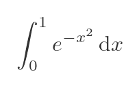
Here is how we would use the quad function to find the approximate value of the integral above:

import numpy as np
from scipy.integrate import quad

def f(x):
    return np.exp(-x**2)

integral, error = quad(f, 0, 1)
print(integral, error)  # 0.7468241328124271, 8.29e-15

After the imports, we define our function f(x). This is the function we wish to integrate. Notice that we use the np.exp (the NumPy exponential function) rather than the regular math.exp function. It is convenient to use NumPy when dealing with arrays of data. NumPy stores large data arrays more efficiently than a Python list, and it can be more efficient if we need to do further processing on the data. However, you can use the regular math functions if you prefer.

We then call quad, passing in the function f, and the upper and lower limits of the integral, which are 0 and 1 as defined above.

The quad function returns two values, as a tuple. The first is the calculated value of the integral. The second is an estimate of the absolute error of the result. In our case, the integral evaluates to approximately 0.7468241328124271. The absolute error is 8.29e-15. This means that the result obtained is accurate to about 14 decimal places.

You should always check the error value. It should be very small compared to the integral value. If it is large, this might indicate a problem with the integral. In addition, quad can throw an IntegrationWarning if the integration fails to converge. This is unlikely to happen if you are using ordinary, well-behaved mathematical functions. The official SciPy documentation has more details if you should encounter this warning.

Checking the integral

Here is a graph of the function above, showing the region we are trying to integrate:

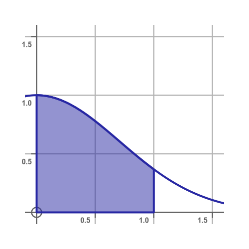
To check the approximate value, we could try to integrate the function mathematically to obtain an exact result. You might recognise this as the famous Gaussian integral.

Unfortunately, this integral doesn't have a simple solution in terms of the standard mathematical functions. Instead, we can calculate the integral like this:

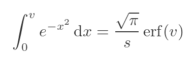
Where erf is the error function, a special function used in certain calculus problems. We are interested in the integral between 0 and 1, so we need to set v to 1:

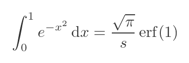
The value of erf(1) is approximately 0.8427007929497149, so we can calculate the integral like this:

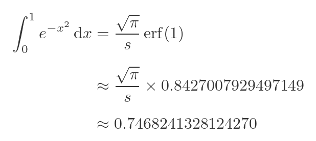
This matches the value from the quad function to 15 decimal places, as expected.

How does quad work?

The quad function approximates the area under the curve by evaluating the function at various points. Here is a much simplified illustration of how it works:

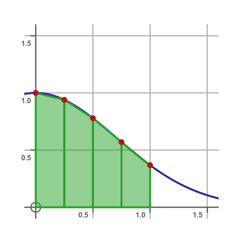
Here, we have calculated the curve's value at 5 points, indicated by the red dots. We have created 4 trapeziums based on those points. We can easily calculate the total area under the trapeziums, which will be approximately equal to the area under the curve, which of course is equal to the definite integral of the curve.

Using four trapeziums will not yield a particularly good approximation, but a computer can easily use far more points to obtain a more accurate one.

In fact, the quad function is a lot more sophisticated than the simple example above. The Fortran QUADPACK library uses a technique called adaptive Gauss-Kronrod quadrature. It is not necessary to understand all the details to be able to use the function, but out of interest here is an overview of how it works:

• It doesn't use trapeziums, instead it attempts to fit a polynomial to the curve, which gives a far more accurate approximation to the curve.
• It also uses advanced techniques to estimate how accurately each slice represents the area under the real curve.
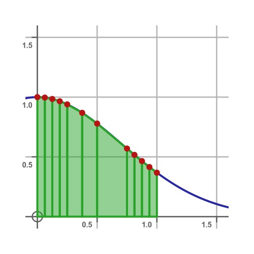
• Using the estimates for each slice, it subdivides each slice just enough to achieve the required accuracy.

This means that the slices might not all be the same width, like this:

More features of the quad function

There are some additional features of the quad function:

• Support for improper integrals.
• Support for functions that have singularities or discontinuities.
• Special handling for integrands that take particular forms (weights).

We will cover these below.

Support for improper integrals

An improper integral is an integral that violates the usual assumptions of a definite integral. The most common example is when one or both of the limits is infinite, such as this:

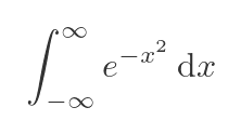
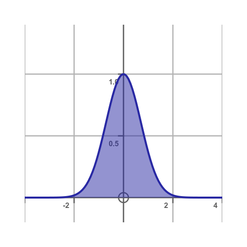
This is actually the famous Gaussian integral. Even though the bounds of the integral are infinite in both directions, the integrand goes towards zero as x tends towards +/- infinity, and in fact the area under the curve is finite. Here is the graph:

We can calculate an improper integral in the usual way, except that we use np.inf (NumPy's definition of infinity) like this:

def f(x):
    return np.exp(-x**2)

integral, error = quad(f, -np.inf, np.inf)
print(integral, error)  # 1.7724538509055159 1.4202636780944923e-08

The Gaussian integral is famously equal to the square root of pi, around 1.772453851, which is the result we get. Notice that this time the result is accurate only to about 8 decimal places. This is because an indefinite integral is harder to calculate to a very high degree of accuracy.

Integrals with discontinuities or singularities

This integral has a singularity at 0:

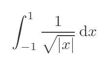
For positive x, this function is equal to 1 divided by the square root of x, which goes to infinity as x goes to zero. Since we are taking the modulus of x, the function is just reflected over the y-axis. Here is a graph of the function, with the area to be integrated shown shaded:

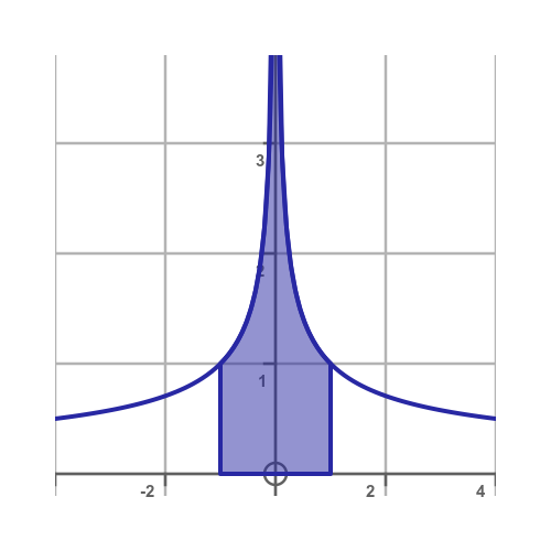
Even though the function goes to infinity, the area under the curve is finite. However, we can't just use quad on this function, because quad might try to evaluate it at zero, which would fail. Instead, we must warn quad that there is a singularity. We do this by passing in an extra parameter, points, which takes a list of any special points, such as singularities or discontinuities, so quad can work around them.

def f(x):
    return 1/(np.sqrt(np.abs(x)))

integral, error = quad(f, -1, 1, points=[0])

In our case, we have only one troublesome point at x = 0, but if there are multiple special points, they can be added to the list.

Special handling for particular integrands

quad has special handling for integrands that take particular forms. This is optional, but it allows quad to calculate the integral more efficiently, and potentially more accurately.

Here is an example, if we wish to find:

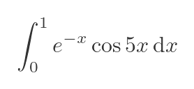
We can use quad to calculate this, in the normal way:

quad(lambda x: np.exp(-x) * np.cos(5*x), 0, 1)

But we can also express the integral like this:

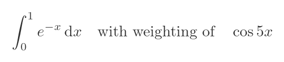
The weighting function is multiplied by the integrand before integrating, so this gives the same integral as before. However, in Python we can specify the weight function explicitly:

quad(lambda x: np.exp(-x), 0, 1, weight="cos", wvar=5)

Notice that we have removed the cos function from the integrand, but added a "cos" weight function with a wvar parameter of 5 (because the original equation involved cos 5x). This will give pretty much the same result as before (it is not exactly the same because the weighting method is slightly more accurate). But because quad knows that the integral has cos as a factor, it can apply special techniques to calculate the result more efficiently.

We won't go into more detail here. Other weighting functions can be used, such as sin, log, and algebraic expressions. See the SciPy documentation for more details.

The fixed_quad function

The fixed_quad function is an alternative to the quad function that can be useful sometimes. It works similarly, but it uses a fixed number of sample points. By contrast, the quad function is adaptive so it uses as many sample points as required to achieve an accurate result (which depends on the function being integrated). For example:

integral, error = fixed_quad(f, 0, 1, n=100)

This integrates the function f between 0 and 1, taking 100 sample points, as specified by the parameter n. One other difference is that fixed_quad doesn't calculate an estimated error value, so it always returns a value of 0 for error.

fixed_quad is usually faster than quad but often yields slightly less accurate results. It also tends to do worse with tricky integrands because it cannot adapt. Typically you should consider this function when:

• You are dealing with particular integrals that are known to be fairly straightforward.
• You only require a certain level of accuracy, for example you need the result to be accurate to 4 significant figures.
• You want to guarantee that the result will never take longer than expected.

A typical use case might be an application with a real-time aspect. In that case, it is better to have a slightly less accurate result in time than a slightly more accurate result that arrives too late.

Double and triple integrals

We can perform a double integral like this:

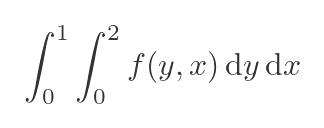
This will find the total volume under the function f(y, x) over the unit rectangular region where 0 < x < 1 and 0 < y < 2. Here is how to express this in Python, using the dblquad function:

from scipy.integrate import dblquad

integral, error = dblquad(f, 0, 1, lambda x: 0, lambda x: 1)

Some important points to notice here:

• The inner integral uses the variable y and the outer integral uses the variable x.
• The function f(y, x) takes the inner variable y as its first parameter and the outer variable x as its second parameter. That is a little unintuitive and can be easy to miss.
• Parameters 2 and 3 are numbers that represent the lower and upper bounds of the outer integral in x.
• Parameters 4 and 5 are functions of x that represent the lower and upper bounds of the inner integral in y.

In this example, parameters 4 and 5 are lambda functions that return the constant values 0 and 1, so the integral evaluates to a rectangular region, as noted above.

Here is a second example:

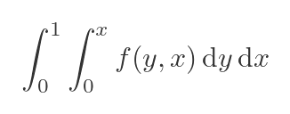
This time the inner integral has bounds that depend on x. This actually integrates over a triangular base area, but we won't go into details here. This integral can be expressed in code as:

from scipy.integrate import dblquad

integral, error = dblquad(f, 0, 1, lambda x: 0, lambda x: x)

All we have changed is the final parameter of dblquad, so now the upper limit of the inner integral is x.

The function tplquad extends this concept to three dimensions. There is also an nquad function that works on n dimensions, but be aware that is has a different call style to dblquad. We won't cover those functions here, refer to the SciPy documentation for more details. Be aware that

Integrating Sampled Data

Sometimes you might not have a function, you might have a table of x, y values. They might come from a sensor, or simulation output, or experiment. scipy.integrate provides tools to estimate the integral of the underlying function directly from discrete samples.

This is called numerical integration, and this article explains some of the maths behind it.

The first function, trapezoid, uses the trapezoidal rule to estimate the area. In other words, it approximates the area under the curve by connecting consecutive points with straight line segments and summing the areas of the resulting trapezoids.

Here is a simple example to integrate a sampled sin function:

from scipy.integrate import trapezoid

x = np.linspace(0, np.pi, 10)
y = np.sin(x)
result = trapezoid(y, x)

This code first generates a NumPy array of x values, using linspace. These values are equally spaced between 0 and pi. It then generates a set of y values corresponding to the value of that function at those points. This graph shows the sample points (x, y) as red dots:

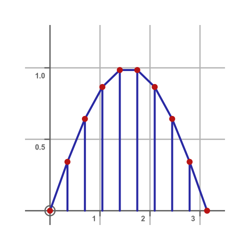
The trapezoid function calculates the area of each trapezoid (shown in blue) and sums them. This gives an approximation to the area under the true curve, the sine function. The diagram uses quite a low sample rate. If we used a much higher sample rate, the sample points would yield a much more accurate estimate of the area.

There are a couple of variants of this function, which we won't cover in detail here, because they work in a similar way to the trapezoid function.

The first is simpson. This uses Simpson's rule to create a more accurate approximation to the curve. Rather than fitting a straight line between each pair of points, it takes the points in sets of 3 and fits a parabola to each set. If the underlying curve is smooth, this can create a significantly more accurate approximation.

The second is cumulative_trapezoid. This function works similarly to trapezoid, but instead of returning just the final area, it returns an array of all intermediate results. This is useful in certain signal processing applications. We won't cover it here, but it is worth being aware of in case you need it. There is also a relatively new cumulative_simpson function available.

Conclusion

The scipy.integrate module provides several useful functions for performing numerical integration. It is useful if you need to:

• Integrate a function that has no easy analytical solution.
• Integrate a function where it might not be convenient to find an analytical solution.
• Integrate a function where the function is unknown and only sampled data is available.

It is based on highly mature and efficient Fortran libraries and features a clean Python API.