The SciPy ecosystem, what it is and why you need it

If you've been writing Python for a while, you've almost certainly used NumPy. You probably know how to create arrays, slice them, broadcast operations across them, and you will appreciate how much faster they are than plain Python lists. But at some point, you might have needed to fit a curve to some data, solve a differential equation, run a statistical test, or similar. You might have found yourself either writing a lot of boilerplate mathematics from scratch or hunting for a specialist library. That specialist library, more often than not, should have been SciPy.

SciPy has been around since 2001, which makes it one of the most mature and battle-hardened libraries in the Python ecosystem. It is used across scientific computing, engineering, data analysis, and research. NumPy gives you the container for numerical data, SciPy gives you the tools to actually do science with it.

This article is the first in a series on SciPy. Here, we'll map out the entire SciPy landscape so you know what's available and where to look when you need it. We'll also clear up common misconceptions and highlight conventions you'll use throughout this series.

Where does SciPy fit?

It helps to think of the scientific Python ecosystem as a layered stack. Each layer builds on the one below it:

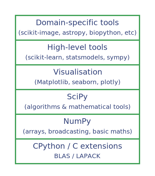
SciPy sits just above NumPy and provides the scientific algorithms (integration, optimisation, signal processing, statistics, and so on). Higher-level libraries like scikit-learn build on SciPy (and NumPy) rather than reimplementing everything themselves.

This means that understanding SciPy well gives you a solid foundation for working with much of the broader Python scientific ecosystem.

What SciPy is not

Before we go further, it's worth clarifying what SciPy doesn't do:

• SciPy is not a machine learning library. For ML, use scikit-learn, PyTorch, or TensorFlow. SciPy provides some statistical and optimisation tools that underpin ML, but it doesn't include classifiers, neural networks, or pipelines.
• SciPy is not a plotting library. It has no built-in visualisation. Use Matplotlib, seaborn, or plotly to visualise your SciPy results.
• SciPy is not a symbolic maths library. It works numerically - with floating-point numbers - not symbolically. For symbolic algebra, use SymPy.
• SciPy is not a replacement for NumPy. SciPy works with NumPy. Most SciPy functions take NumPy arrays as input and return NumPy arrays as output.

Installing SciPy

If you're using a standard scientific Python setup, you probably already have SciPy installed. If not, you can install it with pip:

pip install scipy

Or conda:

conda install scipy

You can verify your installation and check the version like this:

import scipy
print(scipy.__version__)  # e.g. '1.17.1'

The golden rule: how to import SciPy

Here's something that trips up many newcomers. You might expect to do this:

import scipy

scipy.linalg.solve(A, b)  # This will likely fail

But SciPy's submodules are not automatically imported when you import the top-level scipy package. Instead, you should always import the specific submodule you need:

# The correct way - import the submodule explicitly
from scipy import linalg

linalg.solve(A, b)

Or for specific functions:

# Also fine - import just what you need
from scipy.linalg import solve

solve(A, b)

This is a deliberate design decision. SciPy is large, and importing everything would be slow and wasteful. Think of it like importing from a specific drawer in a very large toolbox, rather than tipping the whole thing out onto your workbench.

A map of the submodules

SciPy is organised into 15 submodules. Here's a quick tour, so you have a mental map before we dive into them individually later in this series.

If you are unfamiliar with any of these areas, don't worry at this stage. We will look at them all in later articles.

scipy.linalg - linear algebra

This module provides everything you need for working with matrices and linear systems. This goes beyond numpy.linalg by offering a richer set of decompositions, matrix functions, and direct access to the underlying LAPACK and BLAS routines.

Here is a simple example, using linear algebra to solve a system of simultaneous equations:

from scipy import linalg
import numpy as np

A = np.array([[3, 1], [1, 2]])
b = np.array([9, 8])

x = linalg.solve(A, b)
print(x)  # [2. 3.]

In general, the examples in this section are provided to give a feel for how each submodule is used. It is not necessary to understand every example (for example, if you are not interested in using SciPy for linear algebra, you can ignore this example). Each submodule will be covered in more depth in later articles.

scipy.optimise - optimisation and root finding

Find the minimum of a function, fit a model to data, find where a function equals zero, or solve a linear programming problem. This is one of the most immediately useful modules for practising programmers.

from scipy. optimise import minimise

# Minimise f(x) = (x - 3)^2 + 1
result = minimize(lambda x: (x - 3)**2 + 1, x0=0)
print(result.x)  # [3.]

scipy.integrate - integration and ODEs

Numerically integrate functions and solve ordinary differential equations. Indispensable in physics, engineering, and biology, or anywhere a rate of change needs to be modelled over time.

from scipy.integrate import quad
import numpy as np

# Integrate sin(x) from 0 to pi
result, error = quad(np.sin, 0, np.pi)
print(result)  # 2.0 (exactly, within floating point precision)

scipy.stats - statistics

This module provides a comprehensive statistics toolkit covering probability distributions, descriptive statistics, hypothesis tests, and correlation. If you need to go beyond what Pandas provides, you will probably find what you're looking for here.

from scipy import stats

data = [2.1, 2.5, 2.3, 2.8, 2.0, 2.6, 2.4] 
t_stat, p_value = stats.ttest_1samp(data, popmean=2.5)
print(f"p-value: {p_value:.4f}")

scipy.interpolate - interpolation

Given a set of data points, estimate values in between them. Useful when working with sampled data that you need to resample, smooth, or evaluate at arbitrary points.

from scipy.interpolate import CubicSpline
import numpy as np

x = np.array([0, 1, 2, 3, 4])
y = np.array([0, 1, 4, 9, 16])

cs = CubicSpline(x, y)
print(cs(2.5))  # ≈ 6.25

scipy.signal - signal processing

Filter signals, analyse frequency content, detect peaks, and perform convolution. Used heavily in audio processing, communications, biomedical engineering, and any application involving time-series data.

from scipy.signal import find_peaks
import numpy as np

signal = np.array([1, 3, 1, 4, 1, 5, 1, 4, 1, 3])
peaks, _ = find_peaks(signal, height=3)
print(peaks)  # indices of peaks: [1 3 5 7]

scipy.fft - fast fourier transforms

Transform signals from the time domain to the frequency domain and back again. The FFT is an important algorithm in signal processing, and SciPy's implementation is fast, flexible, and easy to use.

from scipy.fft import fft, fftfreq
import numpy as np

t = np.linspace(0, 1, 500)
signal = np.sin(2 * np.pi * 50 * t)  # 50 Hz sine wave

freqs = fftfreq(len(t), d=t[1] - t[0])
spectrum = fft(signal)

scipy.spatial - spatial data structures

Work with points in space: compute distances efficiently, find nearest neighbours, build Voronoi diagrams, compute convex hulls, and handle 3D rotations.

from scipy.spatial import KDTree
import numpy as np

points = np.random.rand(1000, 2)
tree = KDTree(points)

# Find the 3 nearest neighbours to the point (0.5, 0.5)
distances, indices = tree.query([0.5, 0.5], k=3)
print(indices)

scipy.sparse - sparse matrices

When your matrix is large but mostly zeros (for example, graph adjacency matrices or finite-element systems), storing every element wastes enormous amounts of memory. Sparse matrices store only the non-zero entries.

from scipy.sparse import csr_matrix

# A 5x5 sparse matrix with just 3 non-zero values
row = [0, 1, 3]
col = [0, 2, 4]
data = [1.0, 2.0, 3.0]

M = csr_matrix((data, (row, col)), shape=(5, 5))
print(M.toarray())

This prints:

[[1. 0. 0. 0. 0.]
 [0. 0. 2. 0. 0.]
 [0. 0. 0. 0. 0.]
 [0. 0. 0. 0. 3.]
 [0. 0. 0. 0. 0.]]

Additional modules

The remaining modules are more general-purpose, and we'll dip into them throughout the series:

• scipy.constants - Physical constants (speed of light, Planck's constant, etc.) and unit conversions
• scipy.special - Special mathematical functions: Bessel, Gamma, error functions, orthogonal polynomials
• scipy.ndimage - N-dimensional image filtering, morphology, and geometric transforms
• scipy.io - Read and write MATLAB .mat files, WAV audio, Fortran binary files
• scipy.datasets - Small built-in datasets for testing and experimentation

We will look at a couple of examples. Here is how we might use scipy.constants:

from scipy import constants

print(constants.speed_of_light)     # 299792458.0 (m/s)
print(constants.Planck)             # 6.62607015e-34 (J·s)
print(constants.convert_temperature(100, 'Celsius', 'Kelvin'))  # 373.15

And here is scipy.special, showing the gamma and erf functions:

from scipy.special import gamma, erf
import numpy as np

print(gamma(5))       # 24.0  (i.e. 4!)
print(erf(1.0))       # 0.8427... (the error function, used everywhere in statistics)

A complete example

Let's bring a few things together to show how naturally SciPy fits into a real workflow. Suppose you're analysing some experimental data where you know the underlying model should follow a decaying exponential, but your measurements are noisy.

import numpy as np
from scipy. optimise import curve_fit
from scipy.stats import pearsonr

# --- Simulate some noisy experimental data ---
rng = np.random.default_rng(42)
t = np.linspace(0, 5, 50)
true_signal = 3.0 * np.exp(-0.8 * t)
noisy_data = true_signal + rng.normal(scale=0.2, size=len(t))

# --- Define the model we want to fit ---
def exponential_decay(t, amplitude, decay_rate):
    return amplitude * np.exp(-decay_rate * t)

# --- Fit the model to the noisy data ---
params, covariance = curve_fit(exponential_decay, t, noisy_data, p0=[1.0, 1.0])
amplitude, decay_rate = params

print(f"Fitted amplitude:   {amplitude:.4f}  (true: 3.0)")
print(f"Fitted decay rate:  {decay_rate:.4f}  (true: 0.8)")

# --- Check the quality of the fit ---
fitted_values = exponential_decay(t, *params)
r, p = pearsonr(noisy_data, fitted_values)
print(f"Pearson r:          {r:.4f}")
print(f"p-value:            {p:.2e}")

This outputs something like:

Fitted amplitude:   2.9987  (true: 3.0)
Fitted decay rate:  0.8021  (true: 0.8)
Pearson r:          0.9977
p-value:            3.41e-43

In about 20 lines of clean, readable code, we've simulated an experiment, fitted a mathematical model to noisy data, and statistically validated the fit. No loops to optimise, no manual implementation of least-squares. SciPy handles everything.

A note on performance

You might wonder, if SciPy is written in Python, how can it be fast? The answer is that the heavy lifting isn't written in Python at all. Under the hood, SciPy wraps highly optimised Fortran and C libraries - LAPACK and BLAS for linear algebra, FITPACK for splines, ODEPACK for differential equations, and others. The Python API is a clean and flexible interface to decades of carefully optimised numerical code.

This means you get the best of both worlds, C/Fortran performance with Python convenience. As a rule of thumb, if you find yourself writing a loop to do something mathematical in Python, there's a good chance SciPy already has a vectorised, compiled implementation that will run orders of magnitude faster.

Further reading

• Official SciPy Documentation
• SciPy Lecture Notes - an excellent free textbook
• NumPy - if you want to brush up on the foundations first
• SciPy GitHub Repository - the source code and release notes