Linear gradients in Pycairo

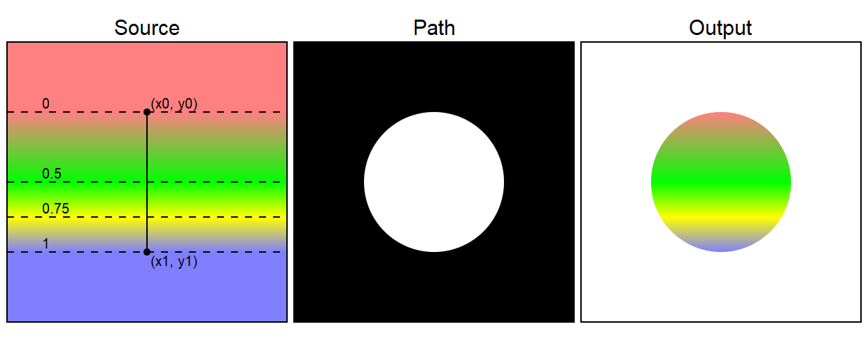
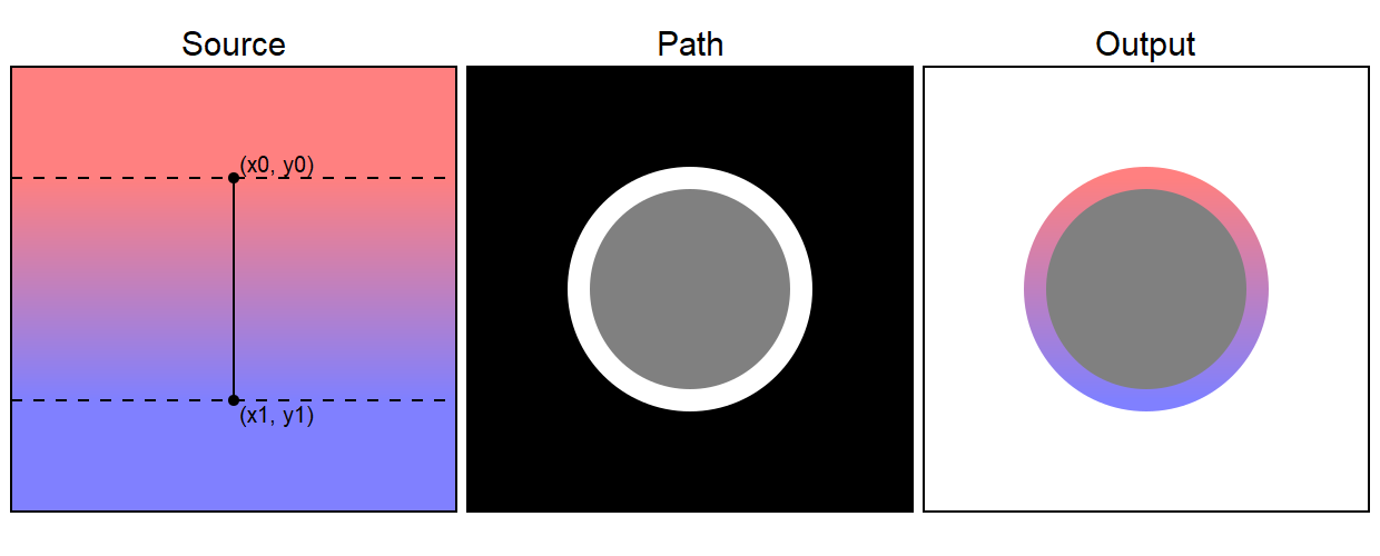
A linear gradient is a gradient that blends smoothly from one colour to another. Here is an example of a circle filled with a linear gradient:

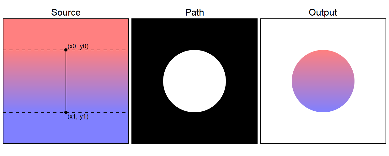
The source is type of object called a pattern - more specifically a LinearGradient pattern. This fills the whole of user space. When this is applied to the path, the resulting output is a circle filled with the gradient. The top of the circle is red, and the bottom of the circle is blue. The colour gradually changes from red to blue as you move down the circle.

Here is the code to draw the gradient:

pattern = cairo.LinearGradient(200, 100, 200, 300)
pattern.add_color_stop_rgb(0, 1, 0.5, 0.5)
pattern.add_color_stop_rgb(1, 0.5, 0.5, 1)
ctx.set_source(pattern)

ctx.arc(200, 200, 100, 0, math.pi*2)
ctx.fill()

The LinearGradient accepts two points (x0, y0) and (x1, y1) that determine the extent of the gradient. In our case we are using the points (200, 100) and (200, 300). These are marked on the source image of the diagram above.

The solid black line from point (x0, y0) to point (x1, y1) defines the direction of the gradient,and also its width. If you draw a band, at right angles to this line, that defined the entire area of the gradient. The gradient is defined between the two dashed lines - this is the area in which the colour varies.

{{% blue-note %}} The area that is outside the gradient band takes a solid colour, (red above and blue below, based on the start and end colours of the gradient). There are other options as we will see later, for example you can make the gradient repeat outside the band. {{% /blue-note %}}

The colour of the gradient is controlled by adding stops. A stop sets the colour at a particular place on the gradient. The rest of the colours are created by interpolating between the stops. The function add_color_stop_rgb takes four parameters:

add_color_stop_rgb(position, r, g, b)

position 0 corresponds to the value of the gradient at the start point (x0, y0), and we set it to an RGB value of (1, 0.5, 0.5) which is a light red.

position 1 corresponds to the value of the gradient at the end point (x1, y1), and we set it to an RGB value of (0.5, 0.5, 1) which is a light blue. We will see later how to add extra stops for multi-coloured gradients.

One important thing to notice is that the position of the control points (x0, y0) and (x1, y1) is defined in the current user space. This makes it easy to create a gradient that extends across the whole circle. We simple chose points that match the top and bottom points of the circle. Since the circle is centred at (200, 200) and has a radius of 100, the points are (200, 100) and (200, 300).

{{% blue-note %}} To be precise, the control points are defined in user space using any transforms that have been applied at the time the gradient is declared. {{% /blue-note %}}

Transparent stops

We can alternatively use the function:

add_color_stop_rgba(position, r, g, b, alpha)

This accepts an additional alpha value to allow transparent stops to be created. The alpha value will interpolate between the stops in the same way as the RGB values.

Linear gradients at different angles

We can change the angle of the gradient by picking two different points. For example, here the points (x0, y0) and (x1, y1) have been moved so that they are diagonally opposite each other:

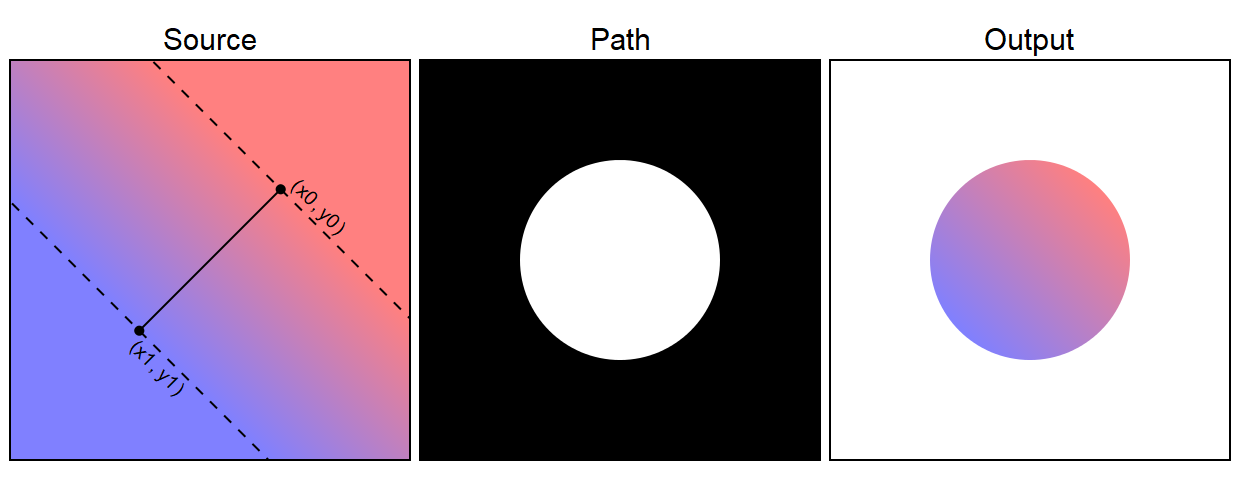
Since the points are now diagonally opposite, rather than one directly above the other, the line joining the points is now at an angle of 45 degrees, meaning that the gradient itself is rotated.

As you can see, this results in a rotated gradient in the output image.

There are two ways to create this gradient. The most obvious one is to calculate the coordinates of the new values of (x0, y0) and (x1, y1). A bit of trigonometry gives these points as approximately (270.7, 129.3) and (129.3, 270.7). Here is the code to draw this:

pattern = cairo.LinearGradient(270.7, 129.3, 129.3, 270.7)
pattern.add_color_stop_rgb(0, 1, 0.5, 0.5)
pattern.add_color_stop_rgb(1, 0.5, 0.5, 1)
ctx.set_source(pattern)

ctx.arc(200, 200, 100, 0, math.pi*2)
ctx.fill()

There is another way to do this. The control points are specified in user space, so if we rotate user space we can create a rotated gradient without the hassle of calculating the new positions of the control points. Here is an example:

# Apply rotation
ctx.save()
ctx.translate(200, 200)
ctx.rotate(math.pi/4)
ctx.translate(-200, -200)

# Define gradient
pattern = cairo.LinearGradient(200, 100, 200, 300)
pattern.add_color_stop_rgb(0, 1, 0.5, 0.5)
pattern.add_color_stop_rgb(1, 0.5, 0.5, 1)

# Restore user space
ctx.restore

# Draw the circle
ctx.arc(200, 200, 100, 0, math.pi*2)
ctx.set_source(pattern)
ctx.fill()

Here we first rotate user space by 45 degrees around the point (200, 200). We use the translate, rotate, reverse translate technique we saw in the Transforms and state chapter earlier.

We then define our gradient. The control points of the gradient take account of the rotated user space.

Finally we restore user space back to its non-rotated state to draw the shape. The shape is drawn non-rotated, but the gradient maintains its rotation because it uses the transform that was in play at the point it was defined.

Adding more stops

Sometimes you might want a gradient that doesn't just transition from one colour to another. You might want move through multiple colours. This can be done using extra stops.

Here is an example:

pattern = cairo.LinearGradient(200, 100, 200, 300)
pattern.add_color_stop_rgb(0, 1, 0.5, 0.5)
pattern.add_color_stop_rgb(0.5, 0, 1, 0)
pattern.add_color_stop_rgb(0.75, 1, 1, 0)
pattern.add_color_stop_rgb(1, 0.5, 0.5, 1)
ctx.set_source(pattern)

ctx.arc(200, 200, 100, 0, math.pi*2)
ctx.fill()

Here is the image it creates:

Stop positions are measured from 0 to 1. In the example:

• The first stop is red and is at position 0, the start of the gradient. Position 0 is the line that passes through (x0, y0).
• The second stop is green and is at position 0.5, halfway down the gradient. The first half of the gradient changes gradually from red to green.
• The third stop is yellow and is at position 0.75, three quarters of the way down the gradient. The third quarter of the gradient changes gradually from green to yellow.
• The final stop is blue and is at position 1, the end of the the gradient. Position 1 is the line that passes through (x1, y1). The last quarter of the gradient changes gradually from yellow to blue.

{{% blue-note %}} Stop positions are clamped between 0 and 1. If you supply a version less than 0 it will be treated as if it were 0, and a version greater than 1 will be treated as if it were 1. {{% /blue-note %}}

Flat colours

Sometimes you might want an area of flat colour in your gradient. Here is an example:

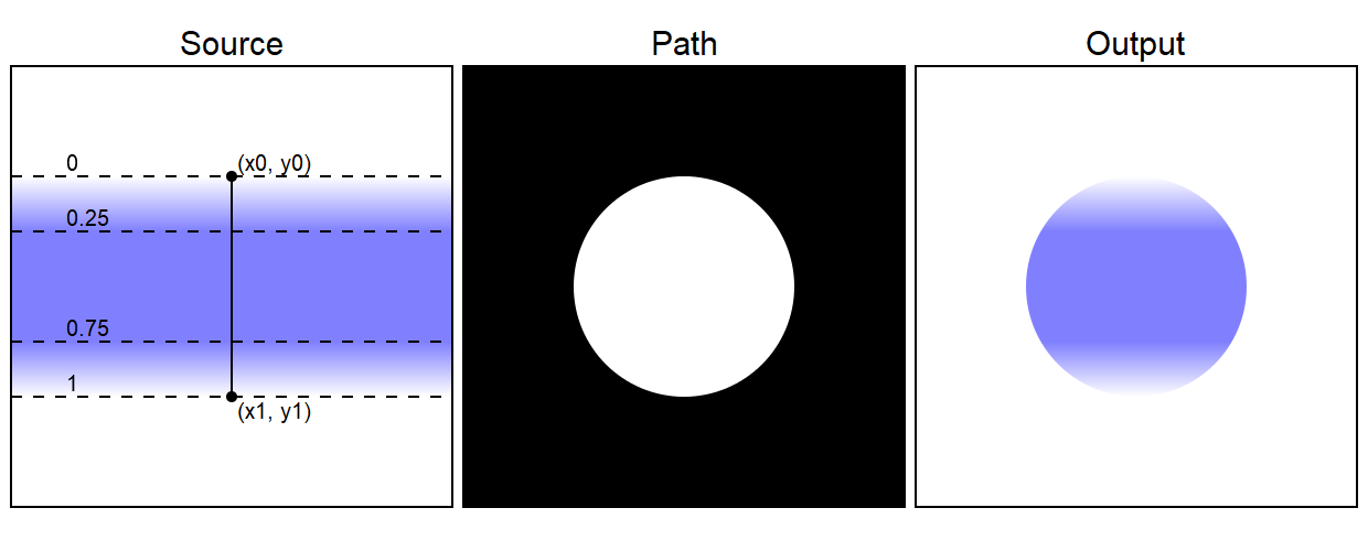
This gradient fades from white to blue, with a band of constant blue in the middle, then fades back to white.

This effect is achieved by setting two consecutive stops to the same colour. In this case the second and third stops (at 0.25 and 0.75) are both set to the same shade of blue, so the central band of the gradient is all one colour:

pattern = cairo.LinearGradient(200, 100, 200, 300)
pattern.add_color_stop_rgb(0, 1, 1, 1)
pattern.add_color_stop_rgb(0.25, 0.5, 0.5, 1)
pattern.add_color_stop_rgb(0.75, 0.5, 0.5, 1)
pattern.add_color_stop_rgb(1, 1, 1, 1)
ctx.set_source(pattern)

ctx.arc(200, 200, 100, 0, math.pi*2)
ctx.fill()

{{% blue-note %}} When you look at the gradient in the output image, it probably appears to have a narrow, darker band horizontally at the 0.25 and 0.75 points. This is an optical illusion. The blue colour is actually constant across the band, then gets lighter towards the top and bottom of the band. However, your eyes can detect a change in the rate of change of the colour and make it appear as an edge. This helps you distinguish object that are a similar colour to their background, but with an artificial computer generated image you end up seeing something that isn't there. {{% /blue-note %}}

Step changes

Sometimes you might want a crisp step-change in colour in a gradient, like the transition from blue to red halfway down this gradient.

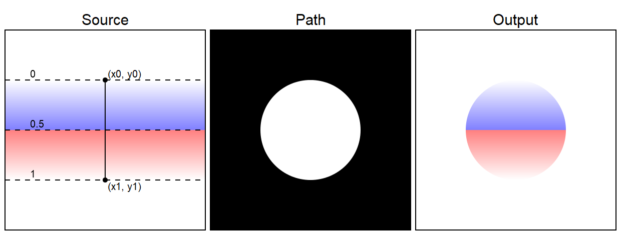
This is formed by 4 stops - white, blue, red and white. However, we don't want a gradual change from blue to red, we want an instant change.

To acheive this, we set the blue and red stops at the same position, 0.5. Pycairo treats the blue stop as the earlier stop, because it is defined first. The red is treated as the later stop because it is defined afterwards. Since they are both in the sane location, the gradient makes a step change. Here is the code:

pattern = cairo.LinearGradient(200, 100, 200, 300)
pattern.add_color_stop_rgb(0, 1, 1, 1)
pattern.add_color_stop_rgb(0.5, 0.5, 0.5, 1)
pattern.add_color_stop_rgb(0.5, 1, 0.5, 0.5)
pattern.add_color_stop_rgb(1, 1, 1, 1)
ctx.set_source(pattern)

ctx.arc(200, 200, 100, 0, math.pi*2)
ctx.fill()

Extend options

A linear gradient defines the colours in a band of user space between the control points (x0, y0) and (x1, y1). Outside that band, Pycairo gives you several options controlling how the colours are extended into the rest of the space:

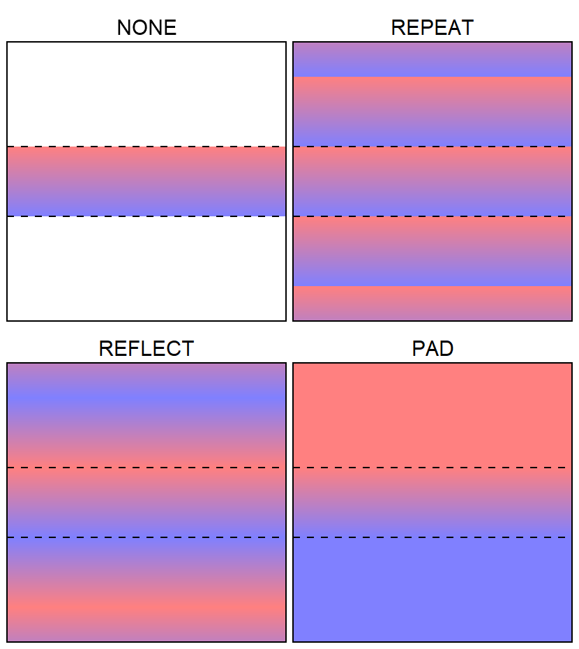
The first option cairo.Extend.NONE only draws the gradient within the band. Outside the band it draws nothing.

cairo.Extend.REPEAT draws the gradient within the band. Outside the band it repeats the same gradient in parallel with the original band.

cairo.Extend.REFLECT is similar to repeat, but each band is reflected. So instead of the bands moving smoothly from red to blue and then making a step change back to red, each alternate band is flipped. The bands move from red to blue, then blue to red, then red to blue and so on.

Finally in cairo.Extend.PAD mode, the pixels outside the band take on the colour of the closest point that is within the band. So every pixel above the gradient ban is red, every pixel below it blue.

The extend mode is controlled by calling the pattern's set_extend function, like this:

pattern.set_extend(cairo.Extend.REPEAT)

The default mode for gradients is PAD.

Filling a stroke with a gradient

Remember that when we apply a stroke to a path, the stroke itself is a shape in its own right. We can paint the stroke with a gradient. It tends to work best with a reasonably thick stroke.

Here is an example:

ctx.arc(200, 200, 100, 0, math.pi*2)
ctx.set_source_rgb(.5, .5, .5)
ctx.fill_preserve()
ctx.set_line_width(20)
pattern = cairo.LinearGradient(200, 100, 200, 300)
pattern.add_color_stop_rgb(0, 1, 0.5, 0.5)
pattern.add_color_stop_rgb(1, 0.5, 0.5, 1)
ctx.set_source(pattern)
ctx.stroke()

In this code we set the source to grey before filling the circle (using set_source_rgb). Then we set the source to a LinearGradient before stroking the shape - this is done in exactly the same way as we previously set the gradient to fill the shape in earlier examples. Here is the result:

We will meet other types of pattern later in this chapter - of course you can paint a stroke with any of the patterns described below.

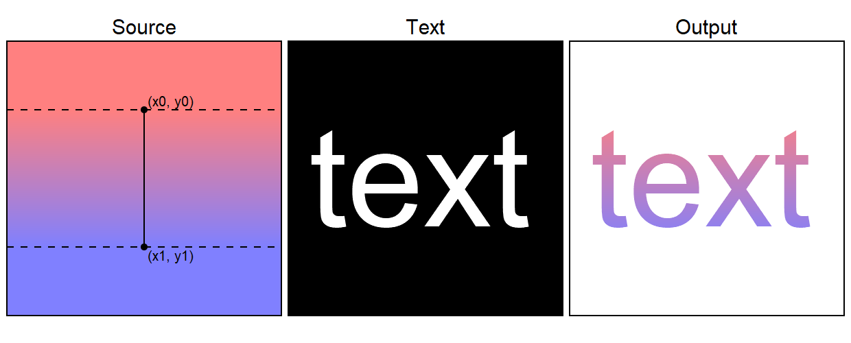
Filling text with a gradient

Filling text with a gradient (or any other pattern described below) is very easy. Simply set the source to the a LinearGradient or other pattern before calling show_text:

pattern = cairo.LinearGradient(200, 100, 200, 300)
pattern.add_color_stop_rgb(0, 1, 0.5, 0.5)
pattern.add_color_stop_rgb(1, 0.5, 0.5, 1)
ctx.set_source(pattern)
ctx.set_font_size(200)
ctx.move_to(30, 270)
ctx.show_text("text")

Here is the result: