Image geometric transforms with NumPy and SciPy

In this section we will see how to use NumPy and to perform geometric transforms on images. For more information on NumPy and images, see the main article.

We saw in the previous article how to perform cropping, padding and flipping on an image. Here we will look at some more complex operations:

• Scaling
• Rotation
• Affine transforms - shearing

NumPy does not provide functions to do these operations. Instead we will use SciPy, which has a an imaging module called ndimage. This module accepts images in NumPy format

Scaling

Here is the code to scale an image. We will scale out image down by 50%:

import numpy as np
from PIL import Image
from scipy import ndimage

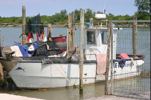
img_in = Image.open('boat.jpg')
array = np.array(img_in)

zoom_array = ndimage.zoom(array, (0.5, 0.5, 1))

img_out = Image.fromarray(zoom_array)
img_out.save('shrink-boat.jpg')

Here we import ndimage from SciPy (you will also need to install SciPy if you don't have it already). We open the image in the usual way.

Here is how we scale the image:

zoom_array = ndimage.zoom(array, (0.5, 0.5, 1))

The zoom function takes a tuple (0.5, 0.5, 1), which specifies that the amges should be scaled by a factor of 0.5 in the first axis (vertical) and second axis (horizontal). This makes the image 50% smaller in height and width.

The third axis represents the 3 colour components of each pixel. We don't want to scale this axis, because we still need 3 colours.

This is the result:

You can vary the scaling factor. (2, 2, 1) makes the image twice as big.

(0.25, 1, 1) reduces the height of the image by a factor of 4, but keeps the original width, like this:

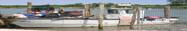
In every case, the third scale factor is 1 to keep the pixel colours unchanged.

Interpolation

Simple operations like padding or flipping an image work by moving pixels around, but they don't affect any individual pixel values. Each pixel in the output image maps onto one particular pixel from the input image.

When we scale an image, this is no longer true. For example, if we make an image 4 times bigger (4 times wider and 4 times taller), the output image has 16 times as many pixels as the input image.

There are two ways we can handle this. We can either replicate each pixel, so that each pixel in the original image gets expanded into a block of 4 by 4 pixels of the same colour. Or we can use interpolation, so that the colour of each output pixel is a weighted average of the neighbouring pixels in the original image.

These two cases are shown here:

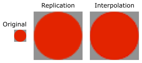
The replication case is quite pixelated. The interpolated case is a lot smoother. It will never be perfect, because interpolation is just an approximation. The aim is to reduce the artificial edges (the 4 by 4 pixels edges), but without blurring the real edge (the edge of the circle).

In fact there are several orders of interpolation. An order of 0 performs no interpolation (it just replicates the pixels). Order 1 to 5 control the degree of interpolation - essentially it controls the number of neighbouring pixels that are used to calculate the value.

You can control the order of interpolation by setting the order parameter to an integer value between 0 and 5. This apples to zoom and the other functions described in this article. It is usually best to stick with the default value of 3 unless you have a good reason to change it. In general:

• Order 0 is faster that the others, but gives poor quality, pixelated results.
• Order 1, 2 or 3 give much better quality, but take a little longer. Higher orders take account of a greater number of nearby pixels in the interpolation. This gives slightly better quality, but take slightly longer to run.
• Higher orders (4 or 5) shouldn't normally be used because they often reduce quality due to over-fitting. They have specialist uses but don't assume they are automatically better than order 3.

On a modern computer, all of these methods will run quite quickly, so it is usually best to stick with the default order 3.

Rotation

Here is the code to rotate an image. We will rotate the image by 45 degrees counterclockwise:

import numpy as np
from PIL import Image
from scipy import ndimage

img_in = Image.open('boat.jpg')
array = np.array(img_in)

rotated_array = ndimage.rotate(array, 45, cval=128)

img_out = Image.fromarray(rotated_array)
img_out.save('rotate-boat.jpg')

Note that the angle is given in degrees not radians.

Here is the result:

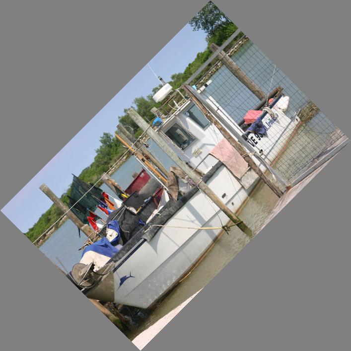
A rotated image is no longer aligned to the x, y axes (unless the angle is a multiple of 90 degrees), so the image ends up with some extra pixels - the black triangles in each corner. The rotate function fills thes areas with zeros. Since the r, g and b values are all set to zero, the resulting colour is black. We can change this using the cval parameter as we will see next.

This image is also larger than the original. We can choose to force the image to be the exact same size as the original by setting reshape to False, like this:

rotated_array = ndimage.rotate(array, 45, reshape=False, cval=128)

Here is the result. The image has been cropped to match the exact size of the original image:

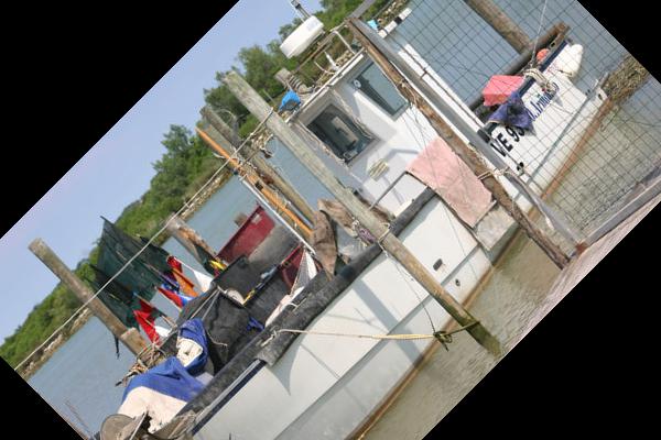
In this example we have also set cval to 128. This parameter controls the value that is used to fill the extra pixels. Insteadof the default zero, we use 128. Again this affects all three colour values r, g, b, so the result is a mid grey. We could have used 255 to give white, of course.

This parameter doesn't allow us to set r, g and b independently, to create a coloured border. The bets way to do that is:

• Pad the original image with a coloured border.
• Rotate the padded image.
• Crop the result to the required size.

You will need to calculate the amount of padding and cropping you need, based on the angle of rotation. That, as they say, is left as an exercise for the reader.

Affine transformations

An affine transformation is a more general transform that can include any of the following types of operation:

• Shifting
• Scaling
• Rotating
• Flipping over any axis
• Shearing
• Any combination of the above

Affine transformations can be defined by a matrix. When a position (x, y) is multiplied by the matrix, it gives a new position (x1, y1). The transformation (in effect) applies this transform to every pixel to obtain a new image.

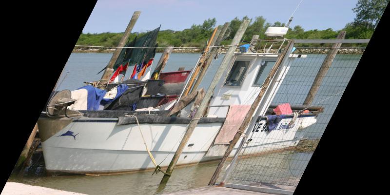
We will give a simple example of a shear transform:

import numpy as np
from PIL import Image
from scipy import ndimage

img_in = Image.open('boat.jpg')
array = np.array(img_in)

height, width, colors = array.shape

transform = [[1, 0, 0],
             [0.5, 1, 0],
             [0, 0, 1]]
sheared_array = ndimage.affine_transform(array,
                                         transform,
                                         offset=(0, -height//2, 0),
                                         output_shape=(height, width+height//2, colors))

img_out = Image.fromarray(sheared_array)
img_out.save('shear-boat.jpg')

An affine transformation can be defined by a matrix:

[[a, b, 0],
 [c, d, 0],
 [0, 0, 1]]

Where a, b, c, d control the rotation, scaling, mirroring and shearing. This assumes no translation. For more details see the Wikipedia entry. The matrix:

[[1, 0, 0],
 [0.5, 1, 0],
 [0, 0, 1]]

Represents a shear of 0.5 in the second dimension (which is the x direction in a NumPy image).

When we call the affine_transform function we also supply an offset value that moves the image so that the leftmost point is at column zero, and an output_shape that tightly contains the output image. Here is the result:

See also

• Image operations with NumPy