Mandelbrot set with generativepy

This article has been moved to my blog. Please refer to that article as it might be more up to date.

The Mandelbrot set is a famous fractal that can be implemented fairly easily with generativepy.

The Mandelbrot set is an escape-time fractal. This article will explain how escape-time fractals work, using the Mandelbrot as an example.

Escape-time fractals

The Mandelbrot set is based on an equation using complex numbers:

znext = z*z + c

Where z is a complex variable, and c is a complex number constant. However, if you are not familiar with complex numbers we can rewrite this equation as a pair of equation in x and y:

xnext = x*x - y*y + c1
ynext = 2*x*y + c2

Where c1 and c2 are two constant values.

Here are those equations implemented in a Python loop:

def calc(c1, c2):
    x = y = 0
    for i in range(10):
        x, y = x*x - y*y + c1, 2*x*y + c2
        print(x, y)

We are interested in what happens as we call this function iteratively, with various values of c1 and c2. Now if we try calling this function with c1 = 0.2 and c2 = 0.1, the sequence of values looks like this:

0.2 0.1
0.23 0.14
0.2333 0.16440000000000002
0.22740153000000002 0.17670904
0.22048537102861931 0.18036781212166242
0.21608125118807261 0.17953692795453008
0.21445759861565283 0.17758912805375543
0.21445416320109933 0.1761706758853121
0.21495448107239606 0.1755610697551134
0.2153837397195433 0.17547527729145027

After a few loops, the seem to stabilise - they converge. We could to run the loop many more times, the values would stay almost the same forever. If we try different values such as c1 = 0.5 and c2 = 1.0, we get something very different:

0.5 0.01
0.7499 0.02
1.06195001 0.039996000000000004
1.6261381437230003 0.09494750519992001
3.135310233727196 0.31879551971385567
10.228539678324857 2.0090457108504634
101.08675928277933 41.10920753800466
8529.065957891833 8311.20313340019
3668869.0894282013 141773599.43841496
-2.0086292897328776e+16 1040297553353152.1

The numbers get very big, very quickly - they diverge. If we ran the loop more times, the numbers would just get bigger and bigger.

The Mandelbrot set

If we try this experiment with lots of different values for c1 and c2, we will find that some values converge and some diverge.

The set of all converging points are called the Mandelbrot set.

Since the equations are so simple, you might expect the shape created by the black pixels to also be simple - maybe a circle or something like that. But in fact the shape is incredibly intricate, the edge of the shape is so complex that you can zoom in on it forever and never run out of finer and finer detail.

To plot this shape, we will first tidy up our calc function:

MAX_COUNT = 100

def calc(c1, c2):
    x = y = 0
    for i in range(MAX_COUNT):
        x, y = x*x - y*y + c1, 2*x*y + c2
        if x*x + y*y > 4:
            return i+1
    return 0

For a given pair of values, we iterate the function MAX_COUNT times. Each time through the loop it checks if the value x*x + y*y is greater than 4. That is the point of no return for the Mandelbrot equations, if that value is exceeded then it is never coming back, it is definitely going to diverge. In that case we return the loop count plus 1, which will be between 1 and MAX_COUNT.

However, if the exit condition hasn't happened within MAX_COUNT attempts, we will assume that it is never going to happen. The calculation has converged, the loop ends, so we return 0 to indicate that (c1, c2) is part of the Mandelbrot set.

Plotting the image

We could make a 2 dimensional plot of all the points in the Mandelbrot set. For each pixel at position (x, y):

• Setting c1 = x and c2 = y, check if the sequence diverges.
• Make the point (x, y) black if the converges, and white if it diverges.

We simply repeat that procedure for every pixel in the image, and plot the result.

It turns out that the interesting part of the Mandelbrot set is in a a region that is 3 units square, with its bottom corner at (-2, -1.5). In other words, x values between -2 and +1, and y values between -1.5 and +1.5. We would like to create an image 600 pixels square that represents this region:

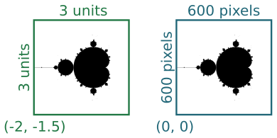
The two squares represent the same region, measured in different coordinate spaces We call the first set (the 3 by 3 square) our user space, and the second set (the 600 by 600 square) our pixel space.

We will use a Scaler object to convert between user space and pixel space. We create the scaler using the parameters above, then we can simple call:

x, y = scaler.device_to_user(px, py)

to convert pixel coordinates to user coordinates.

The drawing code

Here is the full drawing code:

from generativepy.bitmap import Scaler
from generativepy.nparray import make_nparray

MAX_COUNT = 256

def calc(c1, c2):
    x = y = 0
    for i in range(MAX_COUNT):
        x, y = x*x - y*y + c1, 2*x*y + c2
        if x*x + y*y > 4:
            return i+1
    return 0


def paint(image, pixel_width, pixel_height, frame_no, frame_count):
    scaler = Scaler(pixel_width, pixel_height, width=3, startx=-2, starty=-1.5)

    for px in range(pixel_width):
        for py in range(pixel_height):
            x, y = scaler.device_to_user(px, py)
            count = calc(x, y)
            if count==0:
                image[py, px] = 0

make_nparray('mandelbrot-bw.png', paint, 600, 600, channels=1)

First looking at the top level, we are using the make_nparray function to create a bitmap image. This function accepts a paint function that does the actual drawing. The paint function is called with a NumPy array as its first parameter. Since we have defines the image to have one channel (ie a greyscale image) we only need to set one byte value for each pixel

Within the paint function we create a Scaler object using the pixel width and height, and the user space width and offsets as mentioned above.

Now we have the main loop, which loops over every pixel in the output image. On each pass through the loop, px and py indicate the pixel coordinates of the current pixel. Here is the body of the main loop:

x, y = scaler.device_to_user(px, py)
count = calc(x, y)
if count==0:
    image[py, px] = 0

First we use the scaler to convert the pixel coordinates into use coordinates. px which has a range 0 to 599 is converted to a use range of -2.0 to +1.0. py which also has a range 0 to 599 is converted to a use range of 1.5 to -1.5.

We call calc to find out if the point is within the Mandelbrot set. Recall that the value is 0 for points that are in the set, and greater than zero for points outside. We set col to black or white depending on the count.

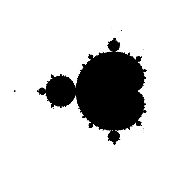
Finally we set the value of the pixel array to 0 (black) if the count is zero. Since the array is initialised to values of 255 (white) we don't need to set the value for pixels that are outside the set.

Here is the image created:

MAX_COUNT

Most of the points that are outside the Mandelbrot set will diverge very quickly. It will only take a few iterations for the value to reach the point where x*x + y*y is greater than 4, so we know for certain it has diverged.

Generally, the closer a point is to the boundary of the set, the longer it will take to diverge. Points that are very close to the border might take a large number of iterations to fully escape. In fact, there is no real limit to how many iterations it might take.

To avoid potentially looping for a very long time, we set a maximum number of iterations. If the point hasn't diverged after that number of iterations, we assume it is part of the set.

A MAX_COUNT of 256 is perfectly good for the whole fractal in a 600 pixel image. If you decided to zoom in to a small part of the fractal, you might see some blockiness around the edge of the fractal. If that happens you can increase MAX_COUNT.

See also

• Tinkerbell fractal with generativepy
• Coloured tinkerbell fractal with generativepy
• King's dream fractal with generativepy
• Gingerbread man fractal with generativepy
• Coloured Mandelbrot set with generativepy
• Burning ship fractal with generativepy