Introduction to computer sound
Categories: sound synthesis
This article gives a very simple introduction to the basics of computer sound, using Audacity, a free, open source sound editor.
You can download it from audacity.org, and it can be used on Windows, Mac or Linux.
We will use it in this section to introduce some basic concepts, but Audacity is a very useful program to have around anyway.
A simple sound
If you open Audacity, it will create a new empty track. Select The Generate | Tone... menu item and this Tone Generator dialog box will appear:
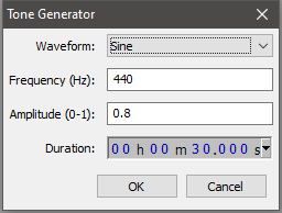
If you hit OK with the settings shown (which are the defaults), it will generate a signal like this:
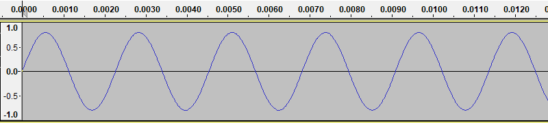
You can play the sound using the play button on Audacity. The sound is 30 seconds of a single musical note (actually the A below middle C).
This particular wave is called a sine wave, because it has the shape of the mathematical sine function. We often use a sine wave as the basic oscillator function because many systems (such as a pendulum or a simple plucked string) can be mathematically modelled by a sine function.
The tone has 3 basic attributes - its amplitude (ie how loud it is), frequency and the shape of the wave. We will look at those next.
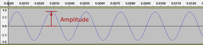
Amplitude
The sound wave we generated has an amplitude of 0.8. This means that the sound wave oscillates between +0.8 and -0.8 (where 1.0 represents the largest possible value):
If we use Audacity to generate a new tone, with the amplitude set to 0.4, we get a waveform like this:
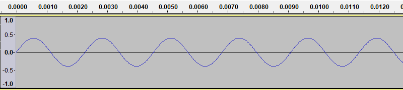
As you might guess, this sound is quieter than the previous one.
The loudness we hear is based on the energy of the signal. Different wave shapes have different amounts of energy, even at the same amplitude, so for example a saw wave (that we will see later) sounds louder than a sine wave at the same amplitude, because carries has more energy.
Frequency
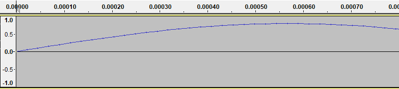
Our simple sine wave repeats the same shape, over and over. We call it a periodic function. The period is the time in seconds between two successive waves. We will measure this between the peaks of the wave:
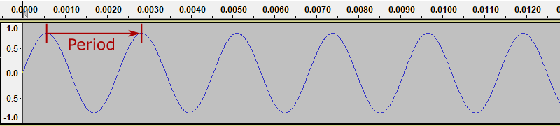
The horizontal scale is in seconds. The from the diagram you can see that period is about 0.0023 seconds (it is actually exactly 0.0022727 recurring).
We normally talk about the frequency of a sound - the number of cycles per second. Frequency is usually measured in Hertz, abbreviated to Hz. 1 Hz means 1 cycle per second. 1 kHz (kilohertz) is 1000 cycles per second. Frequency and period are inverses of each other:
frequency = 1 / period
period = 1 / frequency
In this case we asked Audacity to create a signal with a frequency of 440 Hz, resulting in a period of 0.0022727... seconds.
If we use Audacity to generate a new tone, with the frequency set to 880 Hz, we get a waveform like this:
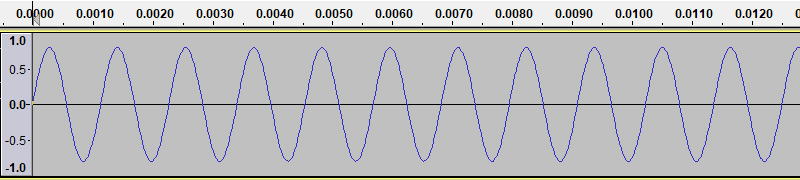
Here you can see that each cycle if half the length of the 440 Hz case, so there are twice as many cycles per second.
The frequency of the sound determines the pitch that we hear. For example, every musical note has its own frequency. The higher the frequency, of course, the higher the pitch.
The human ear can detect sounds with frequency between about 20 Hz and 20,000 Hz. This varies from person to person, and we tend to lose the ability to hear very high frequencies as we get older.
Shape
The wave shape also affect the sound. If you hear a sound with the same frequency but a different shape, it will sound similar but different - like hearing the same musical note played on a different type of instrument.
Here is an example of a saw wave (again created with Audacity, selecting a different waveform in the Tone Generator dialog.):
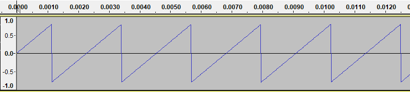
This wave sounds more brassy than a sine wave, and will sound louder than a sine wave of the same amplitude. This is due to the fact that saw wave contains rapid changes, whereas the sine wave is very smooth. Rapid changes correspond to high frequency components of the sound, and of course more energy, which makes the sound louder.
Time varying sounds
So far we have only looked at sounds that remain unchanging for their whole duration.
The most interesting sounds don't stay the same for long. In speech and music, for example, the sound usually changes continuously in various different ways:
- A note played on a piano starts loud but the volume gradually decays.
- A song played on a single instrument consists of a sequence of notes of different frequencies, played on after another.
- Some instruments change timbre even as a single note is played. A sustained note played on a trumpet, for example, often gets "brighter" towards the end.
- Speech is made up of a sequence of varied, complex sounds that can change several times a second, conveying both words and emotion.
- A piece of music will often be made up of several instruments and voices, played at the same time.
The movement of sound over time is undoubtedly the most complex and interesting aspect of sound synthesis.
Sample rate
So far we have looked at sound graphs as if they were continuous functions. But now lets zoom in (Audacity lets you do that with your mouse wheel):
We have zoomed in on the first part of the first cycle of the wave in our original sine wave.
The thing to notice is the small vertical tick marks on the curve. These mark the sample points. When a computer stores a sound, it only stores the values of the signal at the sample points. The curve that Audacity draws is formed by interpolating between these points - in other words, Audacity draws straight lines between the sample points to represent the signal.
A computer sound file (such as a WAV file) is basically a list of numbers, representing the value of the signal at each sample point. When you play a sound file, your computer hardware converts that list of samples into a continuously varying voltage, interpolating in a similar way to Audacity does it draws the curve. This voltage drives your speakers or headphones to create the sound.
We usually sample sounds at a rate of 44,100 samples per second. This is well above the maximum audible frequency of 20 kHz, so it gives reasonable quality.
Sound files normally store sound samples as integer values, because they take up less space and are faster to process. The values on the graphs are floating point values between +1.0 and -1.0. When these values are stored to file, they are usually converted to 16-bit integer values, with a range of +32767 to - 32767. This means that samples are multiplied by 33767 then rounded to the nearest integer, which leads to a tiny loss of precision, but not usually noticeable.
This type of audio, using 44,100 Hz sampling and 16 bit precision, gives quality that is roughly comparable to a CD.
Professional studio recording often uses a sample rate of 88,200 samples per second or higher, and stores each sample as a 24-bit or 32-bit integer. This gives more precision so that sounds can be mixed and resampled without introducing noticeable noise.
Join the GraphicMaths/PythonInformer Newsletter
Sign up using this form to receive an email when new content is added to the graphpicmaths or pythoninformer websites:
Popular tags
2d arrays abstract data type and angle animation arc array arrays bar chart bar style behavioural pattern bezier curve built-in function callable object chain circle classes close closure cmyk colour combinations comparison operator context context manager conversion count creational pattern data science data types decorator design pattern device space dictionary drawing duck typing efficiency ellipse else encryption enumerate fill filter for loop formula function function composition function plot functools game development generativepy tutorial generator geometry gif global variable greyscale higher order function hsl html image image processing imagesurface immutable object in operator index inner function input installing integer iter iterable iterator itertools join l system lambda function latex len lerp line line plot line style linear gradient linspace list list comprehension logical operator lru_cache magic method mandelbrot mandelbrot set map marker style matplotlib monad mutability named parameter numeric python numpy object open operator optimisation optional parameter or pandas path pattern permutations pie chart pil pillow polygon pong positional parameter print product programming paradigms programming techniques pure function python standard library range recipes rectangle recursion regular polygon repeat rgb rotation roundrect scaling scatter plot scipy sector segment sequence setup shape singleton slicing sound spirograph sprite square str stream string stroke structural pattern symmetric encryption template tex text tinkerbell fractal transform translation transparency triangle truthy value tuple turtle unpacking user space vectorisation webserver website while loop zip zip_longest